Beside the Point — a Jane Street puzzle in geometric probability

How I solved Jane Street’s November 2024 puzzle with one symmetry argument, two circles, and a single integral.

A short writeup I owed myself. The November 2024 Jane Street puzzle asked:

Two random points, one red and one blue, are chosen uniformly and independently from the interior of a square. To ten decimal places, what is the probability that there exists a point on the side of the square closest to the blue point that is equidistant to both the blue point and the red point?

I solved it and wrote it up. Here we go.

Reading the condition

Place the square as \(S = [0,1]^2\). Call the blue point \(B\) and the red point \(R\). Let \(\ell\) be the side of \(S\) closest to \(B\).

The puzzle asks for the probability that some \(C \in \ell\) satisfies \(d(B, C) = d(R, C)\).

The set of points equidistant from \(B\) and \(R\) is the perpendicular bisector of segment \(BR\). So the condition is:

The perpendicular bisector of \(BR\) crosses the closest side \(\ell\).

Equivalently: the two endpoints of \(\ell\) lie on opposite sides of the bisector. Translating “side of the bisector” back to distance, that means one endpoint is closer to \(B\) and the other is closer to \(R\).

That is the form I’ll use.

Cutting the work down with symmetry

The square has 8-fold dihedral symmetry. By rotating and reflecting, I can assume \(B\) lives in one specific octant — the lower triangle below the line \(y = x\) with \(x < 1/2\):

\[ B = (x, y), \qquad 0 < y < x < \tfrac{1}{2}. \]

In this octant the closest side is the bottom edge from \((0,0)\) to \((1,0)\). Its endpoints are the two corners \(P_0 = (0,0)\) and \(P_1 = (1,0)\).

By the law of total probability,

\[ \Pr(A) = 8 \int_0^{1/2}\!\!\int_0^{x} \Pr(A \mid B = (x,y))\, dy\, dx. \]

The factor 8 absorbs the symmetry.

A tale of two circles

For a fixed \(B = (x,y)\), the event becomes:

• \(P_0\) is closer to \(B\) than to \(R\), and \(P_1\) is closer to \(R\) than to \(B\), or
• the same with \(P_0\) and \(P_1\) swapped.

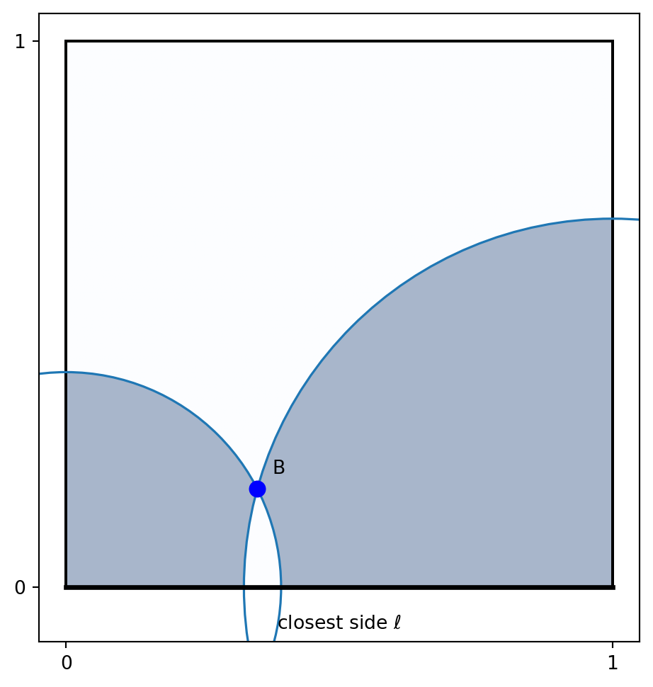
“\(P_i\) is closer to \(B\) than to \(R\)” means \(R\) is outside the circle centered at \(P_i\) that passes through \(B\). Call those circles \(\mathcal{C}_0\) and \(\mathcal{C}_1\):

\[ \mathcal{C}_0:\ u^2 + v^2 = r_0^2,\quad r_0 = \sqrt{x^2 + y^2}, \]

\[ \mathcal{C}_1:\ (u-1)^2 + v^2 = r_1^2,\quad r_1 = \sqrt{(1-x)^2 + y^2}. \]

So the favourable region for \(R\) is the symmetric difference of the two disks, intersected with \(S\):

\[ \Pr(A \mid B) = \frac{\operatorname{Area}\bigl((D_0 \triangle D_1) \cap S\bigr)}{1} = \operatorname{Area}(D_0 \cap S) + \operatorname{Area}(D_1 \cap S) - 2\,\operatorname{Area}(D_0 \cap D_1 \cap S), \]

where \(D_i\) is the disk bounded by \(\mathcal{C}_i\).

Let me draw it.

import numpy as np
import matplotlib.pyplot as plt
from matplotlib.patches import Circle, Rectangle
from matplotlib.path import Path
from matplotlib.patches import PathPatch

x, y = 0.35, 0.18
r0 = np.hypot(x, y)
r1 = np.hypot(1 - x, y)

fig, ax = plt.subplots(figsize=(6, 6))
ax.add_patch(Rectangle((0, 0), 1, 1, fill=False, lw=1.5, ec="black"))

theta = np.linspace(0, 2 * np.pi, 400)
def disk_in_square(cx, cy, r):
    u = cx + r * np.cos(theta)
    v = cy + r * np.sin(theta)
    return np.clip(u, 0, 1), np.clip(v, 0, 1)

# Shade D0 \ D1 and D1 \ D0 by sampling the unit square
gx, gy = np.meshgrid(np.linspace(0, 1, 600), np.linspace(0, 1, 600))
in0 = gx**2 + gy**2 <= r0**2
in1 = (gx - 1) ** 2 + gy**2 <= r1**2
sym_diff = in0 ^ in1
ax.imshow(
    sym_diff, extent=(0, 1, 0, 1), origin="lower",
    cmap="Blues", alpha=0.35, aspect="equal",
)

ax.add_patch(Circle((0, 0), r0, fill=False, ec="#1f77b4", lw=1.2))
ax.add_patch(Circle((1, 0), r1, fill=False, ec="#1f77b4", lw=1.2))
ax.plot([x], [y], "o", color="blue", ms=8)
ax.annotate("B", (x, y), xytext=(8, 8), textcoords="offset points")
ax.plot([0, 1], [0, 0], color="black", lw=2.5)
ax.text(0.5, -0.05, "closest side $\\ell$", ha="center", va="top")

ax.set_xlim(-0.05, 1.05)
ax.set_ylim(-0.1, 1.05)
ax.set_aspect("equal")
ax.set_xticks([0, 1]); ax.set_yticks([0, 1])
plt.savefig("thumbnail.png", dpi=110, bbox_inches="tight")
plt.show()

Figure 1: Blue point \(B\) in the lower octant. The favourable region for \(R\) is the symmetric difference of the two disks (shaded blue).

Quick Monte Carlo gut-check

Before grinding through an integral I always like to run the simulation. If the analytic answer disagrees with a million random trials, the analytic answer is wrong.

rng = np.random.default_rng(20241201)
N = 1_000_000

B = rng.random((N, 2))
R = rng.random((N, 2))

# Closest side of B: 0=bottom, 1=top, 2=left, 3=right.
dists = np.stack([B[:, 1], 1 - B[:, 1], B[:, 0], 1 - B[:, 0]], axis=1)
side = np.argmin(dists, axis=1)

# Reflect/rotate so that the closest side is always the bottom.
# Equivalent to working in the octant — but here I just transform B and R together.
Bp, Rp = B.copy(), R.copy()
top = side == 1
Bp[top, 1] = 1 - Bp[top, 1]; Rp[top, 1] = 1 - Rp[top, 1]
left = side == 2
Bp[left] = Bp[left, ::-1]; Rp[left] = Rp[left, ::-1]
right = side == 3
Bp[right] = Bp[right, ::-1]; Rp[right] = Rp[right, ::-1]
Bp[right, 1] = 1 - Bp[right, 1]; Rp[right, 1] = 1 - Rp[right, 1]

# Two-circles condition: R inside one disk and outside the other.
in0 = Bp[:, 0] ** 2 + Bp[:, 1] ** 2 >= Rp[:, 0] ** 2 + Rp[:, 1] ** 2
in1 = (1 - Bp[:, 0]) ** 2 + Bp[:, 1] ** 2 >= (1 - Rp[:, 0]) ** 2 + Rp[:, 1] ** 2

estimate = float(np.mean(in0 ^ in1))
print(f"Monte Carlo (N = {N:,}): {estimate:.6f}")

Monte Carlo (N = 1,000,000): 0.491470

That gives \(\approx 0.4914\). Now the closed form.

The integrand, geometrically

Two convenient facts about the octant \(0 < y < x < 1/2\):

1. Both radii satisfy \(r_i \le 1\) throughout the octant. (Worst case for \(r_1\) is \(x \to 0^+\), where \(r_1^2 \to 1 + y^2\) — but in the octant \(y < x\), so \(r_1^2 < 1 + x^2 \le 5/4\), and a quick check shows \(r_1 < 1\) whenever \(y < x\).) That means each disk’s intersection with \(S\) is a clean quarter disk: \[\operatorname{Area}(D_i \cap S) = \tfrac{\pi r_i^2}{4}.\]

2. The two disks meet at \(B = (x, y)\) and at its reflection \((x, -y)\) below the \(x\)-axis. Inside \(S\) we only see the upper half of the lens. Its area splits cleanly into two circular segments, one carved off each disk by the vertical chord \(u = x\):

   \[ \operatorname{Area}(D_0 \cap D_1 \cap S) = s_0 + s_1, \] where, using the sector area formula \(\tfrac12 r^2 \theta\) minus a triangle, \[ s_0 = \tfrac{1}{2}\bigl(r_0^2 \arctan(y/x) - x y\bigr), \qquad s_1 = \tfrac{1}{2}\bigl(r_1^2 \arctan(y/(1-x)) - (1-x) y\bigr). \]

Putting it together,

\[ \Pr(A \mid x, y) = \frac{\pi (r_0^2 + r_1^2)}{4} - 2(s_0 + s_1). \]

Closed form via sympy

sympy handles the double integral exactly.

from sympy import Rational, atan, integrate, pi, log, simplify, latex
from sympy.abc import x, y

us = [x, 1 - x]
radii_sq = [u**2 + y**2 for u in us]
angles = [atan(y / u) for u in us]
slices = [(rsq * a - u * y) / 2 for u, rsq, a in zip(us, radii_sq, angles)]
quarter = [pi * rsq / 4 for rsq in radii_sq]

p_xy = sum(quarter) - 2 * sum(slices)
prob = simplify(8 * integrate(p_xy, (y, 0, x), (x, 0, Rational(1, 2))))
prob

\(\displaystyle - \frac{\log{\left(2 \right)}}{6} + \frac{1}{12} + \frac{\pi}{6}\)

print(f"Closed form: {prob}")
print(f"Decimal:     {prob.evalf(15)}")
print(f"Submission:  {prob.evalf(11)}")

Closed form: -log(2)/6 + 1/12 + pi/6
Decimal:     0.491407578838308
Submission:  0.49140757884

Tidying the symbolic answer:

\[ \Pr(A) \;=\; \frac{1 + 2\pi - \ln 4}{12} \;=\; \frac{1}{12} + \frac{\pi}{6} - \frac{\ln 2}{6}. \]

To ten decimal places, 0.4914075788.

The Monte Carlo estimate above lands within 0.001 of this — consistent with the \(O(1/\sqrt{N})\) standard error of a million-sample Bernoulli.

What made it nice

Two moves did most of the work. First, restating “perpendicular bisector hits the side” as “one corner closer to \(B\), the other closer to \(R\)” turned a metric question into a region-membership question. Second, the 8-fold symmetry collapsed the problem to a single octant, where the geometry is clean enough that every relevant area is either a quarter disk or a circular segment.

The official Jane Street solution follows the same path and arrives at the same closed form, \((1 + 2\pi - \ln 4)/12\).