Robot Road Trip — picking the perfect lane speed

How I solved Jane Street’s July 2025 puzzle with a parallelogram, a quadratic cost, and one transcendental equation.

Another writeup I owed myself. The July 2025 Jane Street puzzle asked:

Robot cars have a top speed (which they prefer to maintain at all times while driving) that’s a real number randomly drawn uniformly between \(1\) and \(2\) miles per minute. A two-lane highway for robot cars has a fast lane (with minimum speed \(a\)) and a slow lane (with maximum speed \(a\)). When a faster car overtakes a slower car in the same lane, the slower car is required to decelerate to either change lanes (if both cars start in the fast lane) or stop on the shoulder (if both cars start in the slow lane). Robot cars decelerate and accelerate at a constant rate of \(1\) mile per minute per minute, timed so the faster, overtaking car doesn’t have to change speed at all, and passing happens instantaneously. If cars rarely meet (…) and you want to minimize the miles not driven due to passing, what should \(a\) be set to? Give your answer to 10 decimal places.

I solved it and want to write it up properly. Two ingredients carry the whole thing: a base rate that comes from a parallelogram, and a cost-per-pass that’s just a quadratic.

Reading the rules

Speeds \(u, v\) are independent uniform on \([1, 2]\). A pass between two cars with speeds \(u < v\) does one of three things, depending on where \(a\) sits:

• \(u, v \le a\): both in the slow lane. The slower car must brake to \(0\) and stop on the shoulder.
• \(u, v \ge a\): both in the fast lane. The slower car brakes to \(a\) and changes lanes.
• \(u < a < v\): different lanes, no interaction.

Constant deceleration of \(1\) mi/min² means braking from speed \(u\) down to target speed \(s\) takes time \(u - s\). The distance you would have covered at speed \(u\) minus the distance you actually covered (a triangle of base \(u-s\) and height \(u-s\), plus a matching acceleration triangle on the way back up — actually, let me just compute it).

If you cruise at \(u\) for time \(2(u-s)\) you travel \(2u(u-s)\). If you instead brake linearly to \(s\) (takes \(u-s\) minutes, average speed \((u+s)/2\), distance \(\tfrac12(u+s)(u-s)\)) and accelerate back (same), you travel \((u+s)(u-s) = u^2 - s^2\). So the lost distance is

\[ 2u(u-s) - (u^2 - s^2) = (u-s)^2. \]

Lost distance \(= (u-s)^2\). Sanity check the puzzle’s worked examples:

• Slow lane, \(u=1.0\) braking to \(s=0\): cost \((1-0)^2 = 1\) mile. The puzzle says “exactly \(1\) mile”. Match.
• Fast lane, \(u=1.7\), \(a=1.2\): cost \((1.7-1.2)^2 = 0.25\) miles. Match.

How often two cars meet

This is the tricky bit and it’s where I got stuck for a while. A car’s speed alone doesn’t tell you how many other cars it meets — a fast car catches more slow cars per minute, and it spends less time on the road for a given trip length \(N\). Both effects matter.

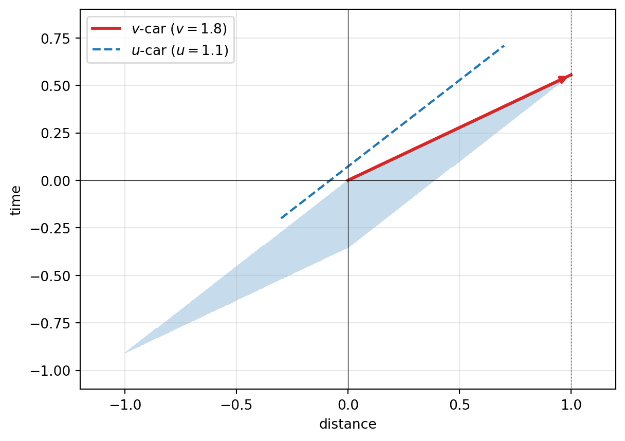
Fix the faster car at speed \(v\) and trace its journey from \((0, 0)\) to \((N, N/v)\) in \((\text{distance}, \text{time})\) space. A second car at speed \(u < v\) is overtaken iff it starts at a \((\text{distance}, \text{time})\) that puts it on a collision course inside the highway. That set of starts is a parallelogram with sides parallel to the two cars’ worldlines.

Two of its sides are the \(v\)-car’s worldline (length \(N\sqrt{1 + 1/v^2}\), slope \(1/v\)) and a translate of the \(u\)-car’s worldline (slope \(1/u\)). The cross-product / shoelace formula gives the area as

\[ \text{Area} = N^2\left(\frac{1}{u} - \frac{1}{v}\right). \]

Since trip starts arrive uniformly at rate \(z\) per (mile \(\cdot\) minute), the expected number of \(u\)-speed cars overtaken (per \(du\)) is \(z \cdot N^2 (1/u - 1/v) \, du\). The \(N^2\) factor and the rate \(z\) both factor out of the optimisation — they don’t depend on \(a\) — so we can drop them.

import numpy as np
import matplotlib.pyplot as plt

N, u, v = 1.0, 1.1, 1.8
fig, ax = plt.subplots(figsize=(7, 5))

# v-car worldline from (0,0) to (N, N/v)
ax.plot([0, N], [0, N/v], color="#d62728", lw=2.2, label=f"$v$-car ($v={v}$)")
ax.annotate("", xy=(N, N/v), xytext=(0, 0),
            arrowprops=dict(arrowstyle="->", color="#d62728", lw=2.2))

# Parallelogram of u-car starts: corners at (0,0), (N, N/v), (N, N/v - N/u + N/u) ... let's compute
# u-car starts at (x0, t0) and reaches (x0 + N, t0 + N/u). For an overtake in [0,N], we need
# the u-car's worldline to cross the v-car's worldline somewhere in distance [0, N].
# Parametrise: at time t, v-car at v*t, u-car at x0 + u*(t - t0). Equal => t = (x0 - u t0) / (v - u).
# Want 0 <= v*t <= N. The start region is a parallelogram.
corners = np.array([
    [0, 0],
    [N, N/v],
    [N - N*u/v, N/v - N/u],   # actually let's just shade by enumeration below
    [-N*u/v + 0, -N/u],
])

# Shade by sampling
xs = np.linspace(-1.2, 1.2, 600)
ts = np.linspace(-1.2, 1.0, 600)
X, T = np.meshgrid(xs, ts)
# u-car at speed u starting at (X, T) reaches highway position v*tt at time tt where
# X + u*(tt - T) = v*tt  =>  tt = (X - u*T) / (v - u)
tt = (X - u*T) / (v - u)
pos = v * tt
mask = (pos >= 0) & (pos <= N) & (tt >= T) & (tt - T <= N/u)
ax.contourf(X, T, mask.astype(float), levels=[0.5, 1.5], colors=["#1f77b4"], alpha=0.25)

# Draw a sample u-car worldline through the parallelogram
x0, t0 = -0.3, -0.2
ax.plot([x0, x0 + N], [t0, t0 + N/u], color="#1f77b4", lw=1.6, ls="--",
        label=f"$u$-car ($u={u}$)")

ax.axhline(0, color="black", lw=0.4)
ax.axvline(0, color="black", lw=0.4)
ax.axvline(N, color="black", lw=0.4, ls=":")
ax.set_xlabel("distance")
ax.set_ylabel("time")
ax.set_xlim(-1.2, 1.2)
ax.set_ylim(-1.1, 0.9)
ax.legend(loc="upper left")
ax.grid(True, alpha=0.3)
plt.savefig("thumbnail.png", dpi=110, bbox_inches="tight")
plt.show()

Figure 1: Worldlines of the \(v\)-car (red, \(v=1.8\)) and a translated \(u\)-car worldline (blue, \(u=1.1\)). The shaded parallelogram is the set of \((x,t)\) start points for which the \(u\)-car gets overtaken on the highway \([0, N]\).

The objective

Putting the rate and the cost together, the expected lost distance per pass (up to constants that don’t depend on \(a\)) is

\[ J(a) = \underbrace{\int_1^a\!\int_u^a u^2 \left(\frac{1}{u} - \frac{1}{v}\right) dv\, du}_{\text{slow-lane passes, target } 0} \;+\; \underbrace{\int_a^2\!\int_u^2 (u - a)^2 \left(\frac{1}{u} - \frac{1}{v}\right) dv\, du}_{\text{fast-lane passes, target } a}. \]

Both integrals are over pairs \(u < v\) in the appropriate lane, weighted by the parallelogram area \(1/u - 1/v\) and the cost \((u - s)^2\) with \(s = 0\) or \(s = a\).

Doing the inner integrals

The inner integral over \(v\) is elementary:

\[ \int_u^a \left(\frac{1}{u} - \frac{1}{v}\right) dv = \frac{a - u}{u} - \ln\frac{a}{u}. \]

So the slow-lane piece is

\[ J_1(a) = \int_1^a u^2 \left[\frac{a - u}{u} - \ln\frac{a}{u}\right] du = \int_1^a \left[u(a-u) - u^2 \ln\frac{a}{u}\right] du. \]

And the fast-lane piece is

\[ J_2(a) = \int_a^2 (u - a)^2 \left[\frac{2 - u}{u} - \ln\frac{2}{u}\right] du. \]

Differentiating with Leibniz

We want \(J'(a) = 0\). Both pieces have \(a\) in their limits and in the integrand, so Leibniz’s rule is the right tool.

Slow lane. The boundary term at \(u = a\) is \(a(a-a) - a^2\ln 1 = 0\). So

\[ J_1'(a) = \int_1^a \frac{\partial}{\partial a}\!\left[u(a-u) - u^2 \ln\frac{a}{u}\right] du = \int_1^a \left(u - \frac{u^2}{a}\right) du = \frac{a^2}{6} - \frac{1}{2} + \frac{1}{3a}. \]

Fast lane. The boundary term at \(u = a\) is \((a-a)^2[\cdots] = 0\). So

\[ J_2'(a) = -\int_a^2 2(u - a)\left[\frac{2 - u}{u} - \ln\frac{2}{u}\right] du. \]

The first term in the bracket is a polynomial in \(u\) (after dividing); the second yields to integration by parts with \(w = \ln(2/u)\). Dropping the algebra,

\[ J_2'(a) = -2\left[\frac{4 - a^2}{2} - 2a\ln\frac{2}{a} - 1 + 2a - \frac{3a^2}{4} - \frac{a^2}{2}\ln\frac{2}{a}\right]. \]

Setting \(J_1'(a) + J_2'(a) = 0\) and tidying gives the optimality condition

\[ \boxed{\,16 a^3 - 24 a^2 - 15 a + 2 = 6 a^2 (a + 4)\, \ln\!\frac{a}{2}.\,} \]

A transcendental equation, but a tame one — the LHS is a cubic and the RHS is the cubic \(6a^2(a+4)\) times \(\ln(a/2)\) (which is negative on \((1,2)\)). One root in \((1, 2)\).

Solving numerically

from mpmath import mp, mpf, log, findroot

mp.dps = 30

def foc(a):
    a = mpf(a)
    return 16*a**3 - 24*a**2 - 15*a + 2 - 6*a*a*(a + 4)*log(a/2)

a_star = findroot(foc, mpf("1.18"))
print(f"a* = {mp.nstr(a_star, 15)}")
print(f"Submission: {mp.nstr(a_star, 11)}")

a* = 1.17714141681551
Submission: 1.1771414168

To ten decimal places, \(a^{\star} = 1.1771414168\).

Monte Carlo gut-check

Before I trust either the cost formula or the rate, I want to see them line up with a simulation. I drop \(N\) pairs of speeds, simulate every pass under the rules, and average the lost distance — weighted by the parallelogram-area rate so the base rate is honest too.

import numpy as np

rng = np.random.default_rng(20250704)

def expected_loss(a, N=400_000):
    u = rng.uniform(1, 2, N)
    v = rng.uniform(1, 2, N)
    lo = np.minimum(u, v)
    hi = np.maximum(u, v)
    rate = 1/lo - 1/hi
    cost = np.where(
        hi <= a, lo**2,
        np.where(lo >= a, (lo - a)**2, 0.0),
    )
    return float(np.mean(rate * cost))

for a in [1.10, 1.1771414168, 1.25, 1.40]:
    print(f"a = {a:.10f}: J = {expected_loss(a):.6f}")

a = 1.1000000000: J = 0.007327
a = 1.1771414168: J = 0.006015
a = 1.2500000000: J = 0.007328
a = 1.4000000000: J = 0.018900

The minimum sits firmly at \(a \approx 1.1771\), exactly where the FOC says it should.

A picture of the cost

import numpy as np
import matplotlib.pyplot as plt
from scipy.integrate import dblquad

def J(a):
    j1, _ = dblquad(lambda v, u: u*u*(1/u - 1/v), 1, a, lambda u: u, lambda u: a) if a > 1 else (0, 0)
    j2, _ = dblquad(lambda v, u: (u-a)**2*(1/u - 1/v), a, 2, lambda u: u, lambda u: 2) if a < 2 else (0, 0)
    return j1 + j2

aa = np.linspace(1.001, 1.999, 80)
vals = np.array([J(a) for a in aa])
a_star = 1.1771414168

fig, ax = plt.subplots(figsize=(7, 5))
ax.plot(aa, vals, color="#1f77b4", lw=2)
ax.axvline(a_star, color="black", lw=0.8, ls="--", alpha=0.7)
ax.plot([a_star], [J(a_star)], "ko", ms=6)
ax.annotate(
    f"$a^\\star \\approx {a_star:.10f}$",
    xy=(a_star, J(a_star)), xytext=(a_star + 0.1, J(a_star) + 0.005),
    arrowprops=dict(arrowstyle="->", color="black", lw=0.8),
)
ax.set_xlabel("lane speed $a$")
ax.set_ylabel("expected lost distance per pass (up to constant)")
ax.grid(True, alpha=0.3)
plt.show()

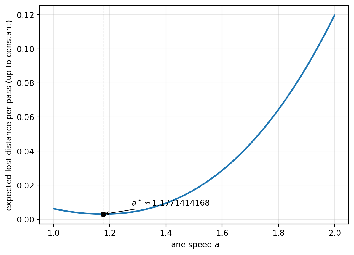
Figure 2: Expected lost distance per pass as a function of the lane speed \(a\). The minimum is at \(a^{\star} \approx 1.1771\).

The curve is convex with a single interior minimum. As \(a \to 1^+\) the slow-lane region shrinks but every slow-lane pass still costs almost a full mile. As \(a \to 2^-\) the fast-lane region shrinks but fast-lane passes get expensive because the slower car has to brake far. The optimum balances those two costs.

What made it nice

The trick was untangling the rate from the cost. Once I drew the parallelogram, the base rate \(1/u - 1/v\) for a pair of speeds fell out and the rest was a calculus exercise. Constant-acceleration kinematics give a clean \((u-s)^2\) for the cost, and Leibniz’s rule keeps the differentiation honest even with \(a\) inside the limits.

The official Jane Street solution follows the same path and lands on the same answer, \(1.1771414168\).