Robot Baseball — tuning the strike zone for maximum drama

How I solved Jane Street’s October 2025 puzzle with one symmetry, a backward induction, and a 1D root-find.

Another writeup I owed myself. The October 2025 Jane Street puzzle asked:

Games are composed of a series of independent at-bats in which the batter is trying to maximize expected score and the pitcher is trying to minimize expected score. An at-bat is a series of pitches with a running count of balls and strikes, both starting at zero. For each pitch, the pitcher decides whether to throw a ball or strike, and the batter decides whether to wait or swing; these decisions are made secretly and simultaneously. (…) An at-bat ends when either the count of balls reaches \(4\) (batter receives \(1\) point), the count of strikes reaches \(3\) (batter receives \(0\) points), or the batter hits a home run (batter receives \(4\) points). (…) Let \(q\) be the probability of at-bats reaching full count; \(q\) is dependent on \(p\). Assume the batter and pitcher are both using optimal mixed strategies and Quad-A has chosen the \(p\) that maximizes \(q\). Find this \(q\), the maximal probability at-bats reach full count, to 10 decimal places.

I solved it and want to write it up properly. The puzzle has two layers: a 2-by-2 game played at every count, and a single dial \(p\) that the league turns to maximise drama. Each layer is short on its own — what makes the puzzle nice is that they fit together cleanly.

Reading the rules

At each pitch the pitcher picks a probability \(t \in [0,1]\) of throwing a strike, and the batter picks a probability \(\sigma \in [0,1]\) of swinging. The four cells of the resulting 2-by-2 give

pitcher  batter	wait	swing
ball	balls \(+1\)	strikes \(+1\)
strike	strikes \(+1\)	home run with prob \(p\), else strikes \(+1\)

An at-bat is a Markov chain on counts \((b, s)\) with \(b \in \{0,1,2,3\}\) and \(s \in \{0,1,2\}\). It terminates when \(b = 4\) (walk, \(1\) point), \(s = 3\) (strikeout, \(0\) points), or a home run (\(4\) points).

Let \(V(b, s)\) be the at-bat value to the batter under Nash equilibrium play. Boundary conditions are \(V(b, 3) = 0\) and \(V(4, s) = 1\).

A symmetry that does most of the work

Write \(V_b = V(b+1, s)\) and \(V_s = V(b, s+1)\). Combining the four cells, the expected payoff at \((b, s)\) is

\[ V \;=\; (1-t)(1-\sigma)\, V_b \;+\; \bigl[t + \sigma - t\sigma(1+p)\bigr] V_s \;+\; 4 p\, t\sigma. \]

Stare at that for a moment. It’s symmetric in \(t\) and \(\sigma\): swap them and nothing changes. The pitcher minimises this and the batter maximises it, but they’re playing against the same expression. So at equilibrium

\[ t^\star = \sigma^\star. \]

That single observation collapses two unknowns per state into one. The Jane Street solution calls it out as the trick: “the outcome of a pitch is symmetric with respect to the pitcher’s choice and the batter’s choice.”

Solving the per-state game

In a mixed-strategy equilibrium of a \(2\times 2\) game, each player picks the probability that makes the opponent indifferent between their two pure actions. From the batter’s side, the batter is indifferent between always waiting (value \(V_b\) if the pitcher’s pitch lands as a ball, \(V_s\) if a strike — overall \((1-t)V_b + t V_s\)) and always swinging (value \((1-t)V_s + t[(1-p)V_s + 4p] = V_s + tp(4 - V_s)\)).

Setting those equal and solving for \(t = \sigma\) gives

\[ \sigma \;=\; \frac{V_b - V_s}{\,4p - (1+p)V_s + V_b\,}. \]

And the equilibrium value (just plug \(t = 0\) into the always-swing expression — both pure actions give the same answer by indifference) is the very tidy

\[ V(b, s) \;=\; V_s + \sigma \cdot p \cdot (4 - V_s). \]

That’s the recursion. Walk the count grid from the terminal states inward and you get \(V\) and \(\sigma\) at every state in twelve assignments.

Counting the path to a full count

Once \(\sigma\) is known at every state, the state-to-state transition probabilities follow from the same payoff matrix. Reading off the cells:

\[ \begin{aligned} \Pr(\text{ball count}\ +1) &= (1-\sigma)^2, \\ \Pr(\text{strike count}\ +1) &= 2\sigma - \sigma^2(1+p), \\ \Pr(\text{home run}) &= p\sigma^2. \end{aligned} \]

(The three add to \(1\), as a sanity check.) Starting from \((0,0)\) with mass \(1\) and pushing forward through this Markov chain, \(q\) is just the mass that lands on \((3, 2)\).

Backward, then forward, in code

import numpy as np

def solve(p):
    """Return q(p) and the equilibrium swing probabilities."""
    V = np.zeros((5, 4))
    V[4, :] = 1.0          # walk
    V[:, 3] = 0.0          # strikeout
    sigma = np.zeros((4, 3))
    for tot in range(5, -1, -1):
        for b in range(4):
            s = tot - b
            if not (0 <= s <= 2):
                continue
            Vb, Vs = V[b+1, s], V[b, s+1]
            sg = (Vb - Vs) / (4*p - (1+p)*Vs + Vb)
            sigma[b, s] = sg
            V[b, s] = Vs + sg * p * (4 - Vs)
    # forward: probability of reaching each state
    q = np.zeros((5, 4))
    q[0, 0] = 1.0
    for tot in range(6):
        for b in range(4):
            s = tot - b
            if not (0 <= s <= 2) or (b, s) == (3, 2):
                continue
            sg = sigma[b, s]
            p_strike = 2*sg - sg*sg*(1+p)
            p_ball = (1 - sg)**2
            q[b, s+1] += q[b, s] * p_strike
            q[b+1, s] += q[b, s] * p_ball
    return q[3, 2], sigma, V

q0, _, V = solve(0.5)
print(f"At p = 0.5: q = {q0:.6f},  V(0,0) = {V[0,0]:.6f}")

At p = 0.5: q = 0.184180,  V(0,0) = 0.919179

A quick sanity check at \(p = 0.5\) — half of swung-at strikes leave the park, which is way too generous for the pitcher. The batter’s expected score should be high, and reaching full count should be unlikely. Both come out as expected.

Optimising \(p\)

We want \(\arg\max_p q(p)\). It’s a one-dimensional problem and \(q\) is smooth on \((0, 1)\), so Brent’s method on the interior is more than enough.

from scipy.optimize import minimize_scalar
from mpmath import mp, mpf

res = minimize_scalar(
    lambda p: -solve(p)[0],
    bounds=(1e-6, 1 - 1e-6),
    method="bounded",
    options={"xatol": 1e-13},
)
p_star = res.x
q_star = -res.fun
print(f"p* = {p_star:.12f}")
print(f"q* = {q_star:.12f}")
print(f"Submission: q* = {q_star:.10f}")

p* = 0.226973229098
q* = 0.295967993374
Submission: q* = 0.2959679934

To ten decimal places, \(q^\star = 0.2959679934\), attained near \(p^\star \approx 0.2269732\).

Monte Carlo gut-check

Before I trust either the recursion or the optimiser, I want to play a few hundred thousand at-bats at the optimal \(p\) and the equilibrium \(\sigma\), and see the empirical full-count rate land on \(q^\star\).

rng = np.random.default_rng(20251004)

def simulate(p, sigma, n=400_000):
    full = 0
    for _ in range(n):
        b = s = 0
        while b < 4 and s < 3:
            if (b, s) == (3, 2):
                full += 1
                break
            sg = sigma[b, s]
            t = rng.random() < sg     # pitcher throws strike with prob sigma
            sw = rng.random() < sg    # batter swings with prob sigma
            if not t and not sw:
                b += 1
            elif t and not sw:
                s += 1
            elif not t and sw:
                s += 1
            else:
                if rng.random() < p:
                    break             # home run
                s += 1
    return full / n

_, sigma_star, _ = solve(p_star)
print(f"Empirical q at p* : {simulate(p_star, sigma_star):.4f}")
print(f"Analytic  q at p* : {q_star:.4f}")

Empirical q at p* : 0.2962
Analytic  q at p* : 0.2960

The two agree to within Monte Carlo noise. Good — both halves of the solver are honest.

A picture of the optimum

import matplotlib.pyplot as plt

ps = np.linspace(0.01, 0.99, 200)
qs = np.array([solve(pp)[0] for pp in ps])

fig, ax = plt.subplots(figsize=(7, 5))
ax.plot(ps, qs, color="#1f77b4", lw=2)
ax.axvline(p_star, color="black", lw=0.8, ls="--", alpha=0.7)
ax.axhline(q_star, color="black", lw=0.8, ls="--", alpha=0.7)
ax.plot([p_star], [q_star], "ko", ms=6)
ax.annotate(
    f"$p^\\star \\approx {p_star:.4f}$\n$q^\\star \\approx {q_star:.10f}$",
    xy=(p_star, q_star), xytext=(p_star + 0.15, q_star - 0.04),
    arrowprops=dict(arrowstyle="->", color="black", lw=0.8),
)
ax.set_xlabel("home-run probability $p$ on a swung strike")
ax.set_ylabel("probability of reaching full count")
ax.set_xlim(0, 1)
ax.set_ylim(0, max(qs) * 1.1)
ax.grid(True, alpha=0.3)
plt.savefig("thumbnail.png", dpi=110, bbox_inches="tight")
plt.show()

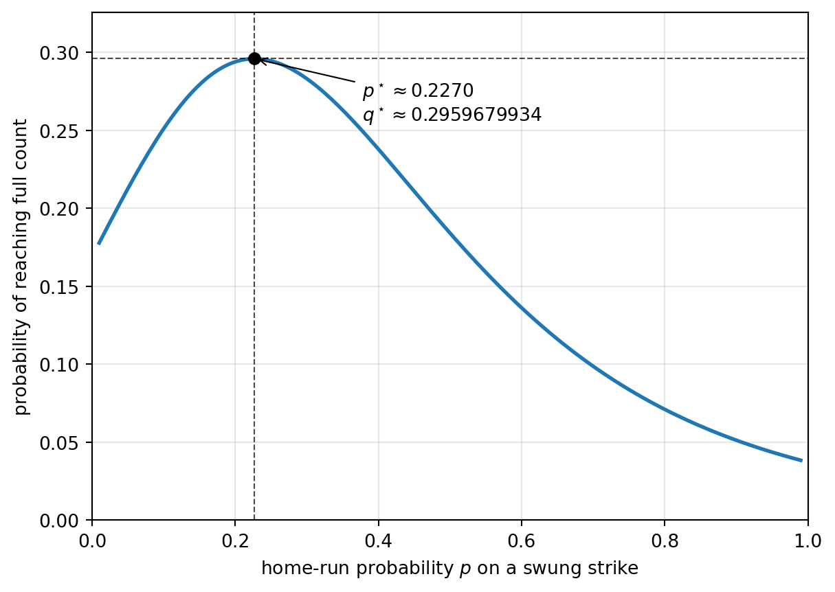
Figure 1: Probability \(q(p)\) of an at-bat reaching a full count, under optimal mixed-strategy play. The maximum sits at \(p^\star \approx 0.227\) with \(q^\star \approx 0.2960\).

The shape makes sense. As \(p \to 0\), batters never bother swinging and pitchers always throw strikes, so at-bats end in three pitches (strikeouts) — full counts are rare. As \(p \to 1\), every swung strike is a home run; batters swing freely and at-bats end fast for the other reason. The sweet spot for length sits in between, just below \(p = \tfrac{1}{4}\).

What made it nice

The trick was the \(t \leftrightarrow \sigma\) symmetry. Once you spot that, every state collapses to a one-variable indifference equation, and the value recursion fits in a few lines of code. Wrapping it in a 1D optimiser over \(p\) does the rest.

The official Jane Street solution follows the same backward-induction-plus-1D-search and lands on the same answer, \(0.2959679934\).